Casio GRAPH 100+ Fonctions supplémentaires - Manuel (Page 151)

20001201
○ ○ ○ ○ ○
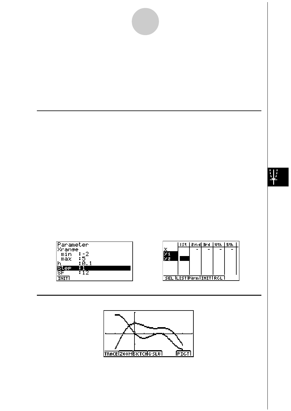
Exemple 1 Représenter graphiquement l’équation différentielle du premier ordre
à deux inconnues suivante.
(
y
1
)
쎾= ( y
2
), ( y
2
)
쎾 = – ( y
1
) + sin x , x
0
= 0, ( y
1
)
0
= 1, ( y
2
)
0
= 0,1, –2 < x < 5, h = 0,1.
Utilisez les réglages de fenêtre d’affichage suivants.
Xmin = –3, Xmax = 6, Xscale = 1
Ymin = –2, Ymax = 2, Yscale = 1
Procédure
1 m DIFF EQ
2 4(SYS)
3 2(2)
4 3( yn )c
w
-3( yn )b+
svw
5 a w
b w
a.b w
6 5(SET)b(Param)
7 -cw
f
w
8 a.b w* 1 i
9 5(SET)c(Output)4(INIT)
cc1(SEL)
(Sélectionnez (
y
1
) et ( y
2
) pour la
représentation graphique.)* 2
i
0 !K(V-Window)
-dw
g
w
b wc
-cw
c
w
b wi
! 6(CALC)
3-5-2
Système d’équations différentielles du premier ordre
* 1 * 2
Ecran de résultat